基于物理的大气散射 (二)

在上一篇文章中，我们根据光照理论传输方程建立了大气散射的物理模型，并给出了数学公式。接下来这篇文章将解释如何求解大气散射积分，以及用代码实现大气散射效果。

[BN08]的论文《Precomputed Atmospheric Scattering》表示可在任意位置实时渲染大气散射效果。论文提出了预结算散射效果放入4D纹理中，在着色器中只需要查找表的消耗来得到当前散射结果，从而提高了渲染效率。

本文接下来也采用预结算的方法先保存散射方程需要的数据，但是不会采用4D查找表的方式，只用采用2D纹理保存即可。

计算散射积分

$L_{In} = \int_{C}^{O}L_{Sun}e^{-T(A(s)->P(s))}e^{-T(P(s)->C)} * V(P(s))(\beta_{R}^{s}e^{-h(s)/H_{R}}p_{R}(\theta)+\beta_{M}^{s}e^{-h(s)/H_{M}}p_{M}(\theta)) ds$

面对此散射积分方程，我们需要用离散的方法去近似求解积分值。首先观察散射方程中的两个光学深度$T(A->P)$和T(P->C)部分，发现光学深度其实就依赖于两个自变量。

* 海拔高度
* 角度：相机方向和太阳方向的夹角。

两个自变量可联想到二维形式，图形学中刚好可以用纹理的U坐标表示高度，V坐标表示角度。

光学深度计算

$T(A->B) = \beta_{R}^{e}\int_{A}^{B}e^{-h(t)/H_{R}dt} + \beta_{M}^{e}\int_{A}^{B}e^{-h(t)/H_{M}dt}$

其中，$\beta_{R}^{e}$和$\beta_{M}^{e}$都是标量，暂时不用管。瑞利散射和米散射在P点到大气层顶部的光学深度积分可预结算出来存在二维纹理。

$T(A->P) = \beta_{R}^{e}.xyzD[h,\cos{\varphi}].x + \beta_{M}^{e}.xyzD[h,\cos{\varphi}].y $

粒子密度

纹理参数化

先考虑UV坐标的数值在[0,1]区间。怎么表示任意高度和任意方向。

任意高度：真实世界的大气高度数值为80000.0f，单位是米。换个思路，用V坐标做插值因子。
任意方向：想象一个圆，任意方向可为单位圆上的一点，因此任意方向可表示为$\cos{varphi}$和$\sin{varphi}$。

1
2
3

float cosAngle = input.uv.x * 2.0 - 1.0;
float sinAngle = sqrt(saturate(1 - cosAngle * cosAngle));
float startHeight = lerp(0.0, _AtmosphereHeight, input.uv.y);

求解交点

刚刚说到我们先计算视线某一点到大气顶端的积分值，但是如何确定终点，即视线与大气层的交点。地球是球体，视线可表示为射线，那么数学上转换就是如何求解直线与球体的交点？

其实也就是初中数学知识，代入法求根运算即可。

float2 RaySphereIntersection(float3 rayOrigin, float3 rayDir, float3 sphereCenter, float sphereRadius)
{
    rayOrigin -= sphereCenter;
    float a = dot(rayDir, rayDir);
    float b = 2.0 * dot(rayOrigin, rayDir);
    float c = dot(rayOrigin, rayOrigin) - (sphereRadius * sphereRadius);
    float d = b * b - 4 * a * c;
    if (d < 0)
    {
        return -1;
    }
    else
    {
        d = sqrt(d);
        return float2(-b - d, -b + d) / (2 * a);
    }
}

密度积分

大气层中的粒子密度不是一层不变，而是随着海波高度的升高，近似呈现为指数衰减。

   intersection = RaySphereIntersection(rayStart, rayDir, planetCenter, _PlanetRadius + _AtmosphereHeight);
   float3 rayEnd = rayStart + rayDir * intersection.y;

// compute density along the ray
   float3 step = (rayEnd - rayStart) / stepCount;
   float stepSize = length(step);
   float2 density = 0;

   for (float s = 0.5; s < stepCount; s += 1.0)
   {
       float3 position = rayStart + step * s;
       float height = abs(length(position - planetCenter) - _PlanetRadius);
       float2 localDensity = exp(-(height.xx / _DensityScaleHeight));

       density += localDensity * stepSize;
   }

大气渲染

因为相机的方向角度，以及太阳的方向都可能实时发生变化，接下来就是如何通过预计算得到的纹理实时渲染出基于物理的大气散射效果。

获取当前点的密度值

上一部分以及得到预计算的密度积分纹理图，只需要通过输入当前点的信息即可得到结果。其中返回结果的x分量是瑞利散射密度积分值，y分量是米散射积分值。

// 输入：_ParticleDensityLUT，[lightZenith, heigh]
void GetAtmosphereDensity(float3 position, float3 planetCenter, float3 lightDir, out float2 localDensity, out float2 densityToAtmTop)
{
    float height = length(position - planetCenter) - _PlanetRadius;
    localDensity = exp(-height.xx / _DensityScaleHeight.xy);  //当前高度的密度

    float cosAngle = dot(normalize(position - planetCenter), -lightDir.xyz);

    densityToAtmTop = tex2D(_ParticleDensityLUT, float2(cosAngle * 0.5 + 0.5, (height / _AtmosphereHeight))).rg;
}

计算当前点的内散射

天空的大气散射除了$T_{CP}$和$T_{AP}$的衰减函数，我们还需要求解当前点的内散射函数。其中与散射系数，密度函数，以及相位函数有关。

void ComputeLocalInscattering(float2 localDensity, float2 densityPA, float2 densityCP, out float3 localInscatterR, out float3 localInscatterM)
{
    float2 densityCPA = densityCP + densityPA;

    float3 Tr = densityCPA.x * _ExtinctionR; //计算瑞利和米散射粒子的光学深度
    float3 Tm = densityCPA.y * _ExtinctionM;

    float3 extinction = exp(-(Tr + Tm));    //当前积分点的消光值

    localInscatterR = localDensity.x * extinction;
    localInscatterM = localDensity.y * extinction;
}

相位函数简单易懂，与波长有关的瑞利散射相位函数，近似均匀向四周发散；与波长无关的米散射相位函数，大概率朝向光源行径方向散射。

//-----------------------------------------------------------------------------------------
// ApplyPhaseFunction[EG2008]
// 瑞利散射和米散射的相位函数
//-----------------------------------------------------------------------------------------
void ApplyPhaseFunction(inout float3 scatterR, inout float3 scatterM, float cosAngle)
{
	// r
    float phase = (3.0 / (16.0 * PI)) * (1 + (cosAngle * cosAngle));
    scatterR *= phase;

	// m
    float g = _MieG;
    float g2 = g * g;
    phase = (1.0 / (4.0 * PI)) * ((3.0 * (1.0 - g2)) / (2.0 * (2.0 + g2))) * ((1 + cosAngle * cosAngle) / (pow((1 + g2 - 2 * g * cosAngle), 3.0 / 2.0)));
    scatterM *= phase;
}

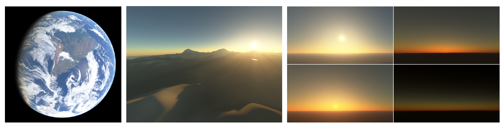
渲染结果

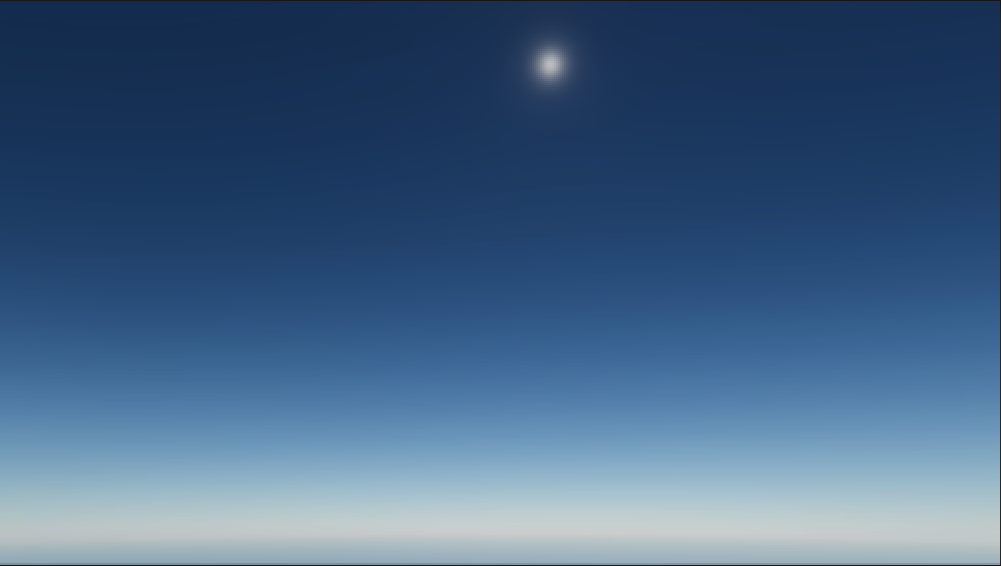
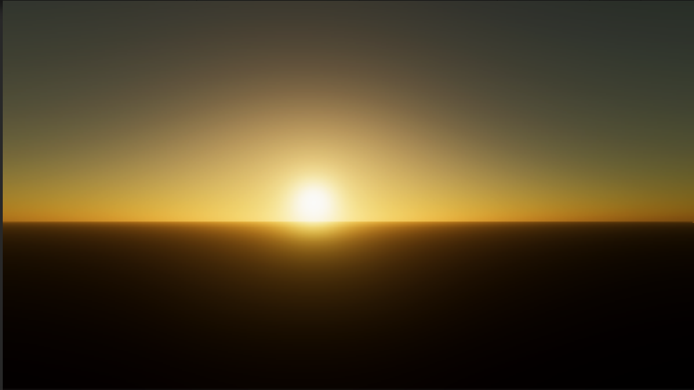
基于物理的太空颜色就是大气层的内散射积分和，求得内散射结果也就是我们的天空背景。而我们的视线路径上的光学深度衰减是密度函数与消光系数乘积结果。

[loop]
   for (float s = 1.0; s < sampleCount; s += 1)
   {
       float3 p = rayStart + step * s;

       GetAtmosphereDensity(p, planetCenter, lightDir, localDensity, densityPA);
       densityCP += (localDensity + prevLocalDensity) * (stepSize / 2.0);

       prevLocalDensity = localDensity;

       float3 localInscatterR, localInscatterM;
       ComputeLocalInscattering(localDensity, densityPA, densityCP, localInscatterR, localInscatterM);
	
       scatterR += (localInscatterR + prevLocalInscatterR) * (stepSize / 2.0);
       scatterM += (localInscatterM + prevLocalInscatterM) * (stepSize / 2.0);

       prevLocalInscatterR = localInscatterR;
       prevLocalInscatterM = localInscatterM;
   }

   float3 lightExtinction = exp(-(densityCP.x * _ExtinctionR + densityCP.y * _ExtinctionM));

大气的消光系数，可用来做大气雾效果，以后的文章将会讲解。

参考资料

GPU Pro 5: High Performance Outdoor Light Scattering Using Epipolar Sampling.
Precomputed Atmospheric Scattering